XGBoost

XGBoost, short for eXtreme Gradient Boosting, is a fast implementation of gradient-boosted decision trees. It builds an ensemble one tree at a time. Each new tree improves the predictions made by the ensemble so far, while regularization and efficient split finding help control complexity and training cost.

A single decision tree is easy to inspect, but may miss useful patterns. A random forest averages many trees trained largely independently. XGBoost instead adds trees sequentially to minimize a chosen loss. That distinction is the core of boosting.

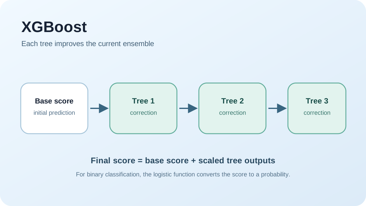
How XGBoost works

1. Start with a base score. For squared-error regression, this is often related to the mean target value. For binary classification, XGBoost works with a raw score, or logit, that is converted to a probability.
2. Measure the current loss. Compute the first and second derivatives of the loss with respect to each current prediction.
3. Grow a new tree. Choose splits and leaf values that improve a second-order approximation to the objective.
4. Add a scaled correction. Multiply the tree output by the learning rate, then update the ensemble's scores.
5. Repeat and validate. Continue until the configured number of trees is reached or an early-stopping rule says to stop.

The new tree does not simply fit the last tree's residuals. It is fitted against the current ensemble using gradients and Hessians of the selected loss.

The model and objective

Let x_i be observation i, b the initial raw score, f_k the output of tree k, and η the learning rate. After K trees, the raw score is:

For regression, this score can be the prediction itself. For binary logistic classification, the predicted probability is σ(F_K(x_i)), where σ is the logistic function.

XGBoost balances fit and tree complexity. With n training examples and K trees, its regularized objective can be written as:

Here ℓ is a task-specific loss, such as squared error or logistic loss. For a tree with T leaves and leaf scores w_j, a common regularizer is:

The parameter γ penalizes each added leaf; λ shrinks large leaf scores. XGBoost can also include an L1 penalty controlled by α; it is omitted from the equations here to keep the split formula readable.

Why gradients and Hessians matter

At boosting round t, define g_i and h_i as the first and second derivatives of the loss at the current raw score F_t−1(x_i):

For a leaf containing examples I, set G = Σ_i∈I g_i and H = Σ_i∈I h_i. Under the L2 regularizer above, the approximate objective is minimized by this leaf score:

To evaluate a candidate split, let G_L, H_L and G_R, H_R be the gradient and Hessian sums in its left and right children. The approximate gain is:

This formula assumes no L1 penalty and a valid candidate split. A positive gain means the split improves the approximate regularized objective. Real training also respects constraints such as minimum child weight and maximum tree depth. The learning rate scales the fitted tree when it is added to the ensemble.

What makes XGBoost practical?

Regularization and pruning. Leaf penalties, a learning rate, depth limits, row and feature sampling, and early stopping can reduce overfitting. They do not guarantee it will never happen.

Efficient split finding. XGBoost can use exact split search or approximate and histogram-based methods. The histogram method bins feature values, reducing the number of candidate thresholds. Work within a tree can be parallelized, even though boosting rounds remain sequential.

Missing values. For a split, XGBoost learns which branch missing values should follow by comparing the gain for each default direction. Missing values are not simply treated as a separate category in every tree.

System optimizations. Cache-aware data access and optional GPU training can make large jobs faster. Actual speed depends on the dataset, hardware, and tree method. Tree growth and split behavior also depend on the chosen configuration; a universal “best split at every level” description would be misleading.

A Python classification example

The UCI Wholesale Customers dataset includes a Channel column. Save its CSV as Wholesale customers data.csv beside your script, then install pandas, scikit-learn, xgboost, and matplotlib. This is a demonstration of the API, not a benchmark claim.

import pandas as pd
import matplotlib.pyplot as plt
from sklearn.metrics import accuracy_score, classification_report, ConfusionMatrixDisplay
from sklearn.model_selection import train_test_split
from xgboost import XGBClassifier, plot_importance

df = pd.read_csv("Wholesale customers data.csv")
X = df.drop(columns="Channel")
y = df["Channel"].map({1: 0, 2: 1})

X_train, X_test, y_train, y_test = train_test_split(
    X, y, test_size=0.3, stratify=y, random_state=42
)

model = XGBClassifier(
    objective="binary:logistic",
    tree_method="hist",
    max_depth=4,
    learning_rate=0.1,
    n_estimators=100,
    reg_alpha=10,
    eval_metric="logloss",
    random_state=42,
)
model.fit(X_train, y_train)
y_pred = model.predict(X_test)

print("Accuracy:", accuracy_score(y_test, y_pred))
print(classification_report(y_test, y_pred, target_names=["Horeca", "Retail"]))
ConfusionMatrixDisplay.from_predictions(y_test, y_pred)
plt.show()

plot_importance(model, importance_type="gain")
plt.show()

The stratified split keeps class proportions similar across training and test sets. The confusion matrix shows which channel labels the model confuses. Gain-based feature importance summarizes how much features improve splits in this fitted model; it is not a causal explanation. For a stronger evaluation, tune on a separate validation set or with cross-validation, then keep the test set untouched until the end.

Advantages and limitations

XGBoost is flexible, often competitive on tabular data, and supports regularization, missing values, parallel split computation, and GPU acceleration. It can still be computationally expensive, especially with large parameter searches. Too many deep trees can overfit, and outliers or mislabeled examples can distort training. The ensemble is also harder to explain than a single tree.

The practical rule is to start with a clear baseline, choose a loss and metric that match the task, and validate the tuned ensemble on data it has not seen. The math tells us how each tree is chosen; held-out performance tells us whether those choices actually helped.